# Vectors and Rasters

(*N.b. this is a refresher from the* [*BAS QGIS Tutorial*](https://lauger.gitbook.io/qgis-tutorial/gis/vectors-and-rasters)*)*

## Vectors

**Vector** data provide a way to represent real world **features** within the GIS environment. A feature is anything you can see on the landscape. Imagine you are standing on the top of a mountain. Looking down you can see rock outcrop, crevasses, lakes, tents and so on (imagining you are in Antarctica!). Each one of these things would be a **feature** when we represent them in a GIS Application. This kind of data is often known as **discrete** data (as opposed to continuous, which we will cover later). Vector features have **attributes**, which consist of text or numerical information that **describe** the features.

A vector feature has its shape represented using **geometry**. The geometry is made up of one or more interconnected **vertices**. A vertex describes a position in space using an **X**, **Y** and optionally **Z** axis.

Vectors are most commonly thought of as **points, (poly)lines and polygons.**

![Example of points, lines and polygons](https://1859916809-files.gitbook.io/~/files/v0/b/gitbook-legacy-files/o/assets%2F-MW-CoufgyGZ3iU5q9S1%2F-MW-azw8VzQbmi8gmrt2%2F-MW007k2A-DiWgaxgCze%2Fimage%20\(6\).png?alt=media\&token=02f4c9ea-ecef-4ce2-b4fa-7626ab8ff59b)

Where there is only a single vertex, it is referred to as a **point**. Examples are station locations, spot heights and ice core locations

Where there are two or more vertices that do not join up at the start and end, a **polyline** is created. Examples are contours, ship tracks and rivers.

Where three or more vertices are present, and the first and last vertex join up, an enclosed **polygon** is created. Examples include land cover, sea ice extent and rock outcrop.

![Diagram explaining the build of points, lines and polygons](https://1859916809-files.gitbook.io/~/files/v0/b/gitbook-legacy-files/o/assets%2F-MW-CoufgyGZ3iU5q9S1%2F-MW-azw8VzQbmi8gmrt2%2F-MW00EzI1ZDTB1jK7Jd8%2Fimage%20\(7\).png?alt=media\&token=8b78e553-b5d4-4406-ac85-b348788785fd)

### Examples of vector data formats <a href="#examples-of-vector-data-formats" id="examples-of-vector-data-formats"></a>

* **Shapefiles**
  * the most common form of vector data within GIS
  * developed and regulated by Esri - proprietary
  * although the term is 'a shapefile', the format actually consists of many different files (between \~3-10), as seen below. You need all of the files for the shapefile to work properly.
* **GeoPackages**
  * a newer and less widespread format for vector data, but with many advantages over shapefiles
  * as seen in the screenshot below, they only consist of one .gpkg file
  * it is defined by the Open Geospatial Consortium (OGC) - therefore open and non-proprietary
* **Geodatabases, GeoJSON, GPX, KML, CSV,** and many more...

![An example of how a geopackage and a shapefile appear in windows explorer](https://1859916809-files.gitbook.io/~/files/v0/b/gitbook-legacy-files/o/assets%2F-MW-CoufgyGZ3iU5q9S1%2F-MW-azw8VzQbmi8gmrt2%2F-MW00O4nRQRg78gzHKvs%2Fimage%20\(8\).png?alt=media\&token=34a2217d-0fdd-4a90-9a1d-2f40d0734c97)

## Rasters <a href="#rasters" id="rasters"></a>

Rasters represent data in a different way to vectors. They are a **grid of pixels**, and each pixel ( sometimes called cells) contains a value that represents the conditions for the area covered by that cell. Some examples of typical raster data include satellite imagery, sea ice concentration and digital elevation models (DEMs).

![A raster, with its matrix of pixels. Each pixel represents a geographical region and each pixel has a value.](https://1859916809-files.gitbook.io/~/files/v0/b/gitbook-legacy-files/o/assets%2F-MW-CoufgyGZ3iU5q9S1%2F-MW-azw8VzQbmi8gmrt2%2F-MW00_1XE26K1WnHTzsy%2Fimage%20\(9\).png?alt=media\&token=28cb65f9-59df-4edf-8afb-378fdc7930c2)

Raster data is used in a GIS application when we want to display information that is **continuous** across an area and cannot easily be divided into vector features. The examples of vector data that we discussed before (station locations, contours, coastline) would be very difficult to represent as a raster. They *could* be saved as a raster, but it would be a big waste of space for all of the pixels that would contain null data.

* It is sometimes sensible to convert data from vector to raster or from raster to vector, but not very often

Rasters should always be **georeferenced** (they should know their place on the earth's surface). This usually consists of a coordinate for the top left pixel in the image, the size of each pixel in the X direction and the size of each pixel in the Y direction. From this information, the file knows the location of each of its pixels.

* Formats for georeferenced rasters can vary. A GeoTiff is a very common format for GIS rasters that has many advantages, but there are many others as well.
* You can sometimes work with non-georeferenced images, for example, old aerial photographs or paper maps that have been scanned. You can add these to your GIS and then manually 'georeference' them by locating common points in the image and in a known dataset.

## How satellite imagery is made?

Remote sensing is the process of detecting and monitoring the physical characteristics of an object by measuring its characteristics at a distance. The measurements taken are usually reflected and emit radiation. For optical imagery, this equals detecting colour and brightness.

The simplest example of remote sensing is taking photos of the Earth's surface from an aircraft or a satellite (with a huge camera).

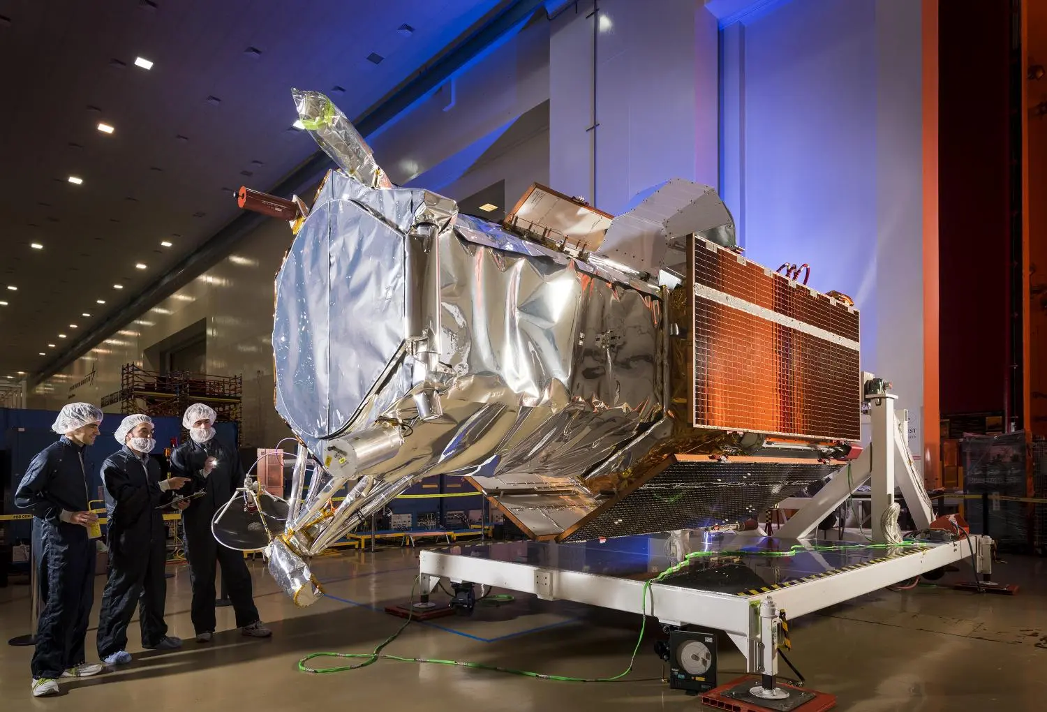
<figure><img src="https://2217084004-files.gitbook.io/~/files/v0/b/gitbook-x-prod.appspot.com/o/spaces%2Fu8dgiMF2h4KnqrWKVkMS%2Fuploads%2FQzzzeZRhhZ9nLwtljrrp%2FWorldView-4-LockMart.webp?alt=media&#x26;token=4b278fd1-cb25-431f-a7dd-26ac1472b056" alt=""><figcaption><p>Digital Globe's WorldView-4 at Lockheed Martin Space Systems' Sunnyvale, California, facility. Credit: Lockheed Martin</p></figcaption></figure>

An example of the most popular use case of satellite imagery would be Google Maps Satellite view.

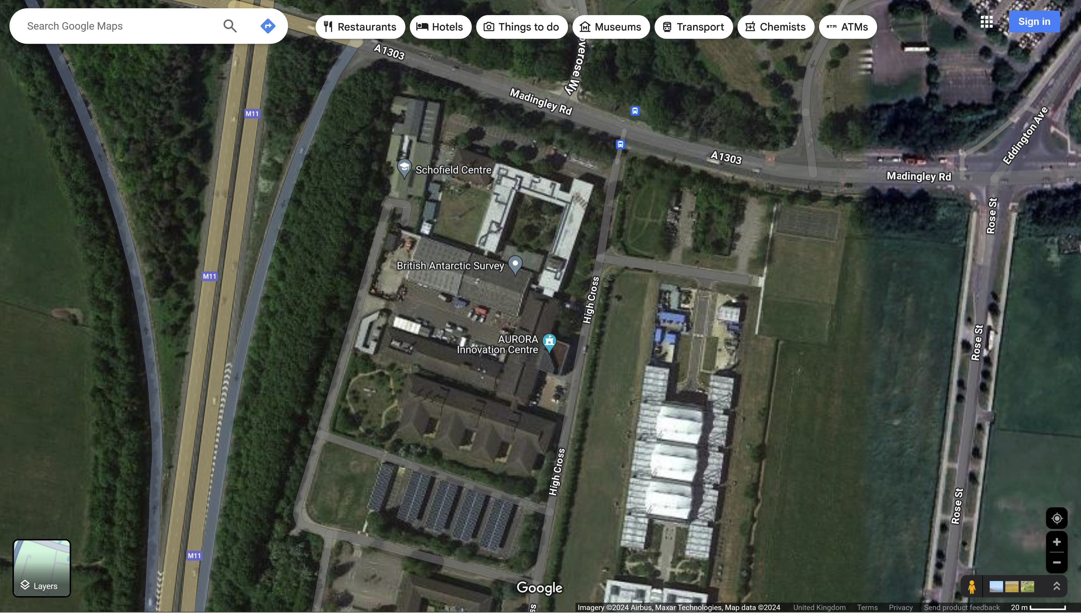
<figure><img src="https://2217084004-files.gitbook.io/~/files/v0/b/gitbook-x-prod.appspot.com/o/spaces%2Fu8dgiMF2h4KnqrWKVkMS%2Fuploads%2FDakIKYjEDD9AIaKfcnU3%2Fimage.png?alt=media&#x26;token=28678a46-f095-4391-9d01-e69fdcc059cd" alt=""><figcaption><p>Satellite view of BAS, Cambridge site. Credit: Google Maps</p></figcaption></figure>

### What types of imagery we usually use?

The most common is to divide sensors into [passive](https://www.earthdata.nasa.gov/learn/backgrounders/passive-sensors), which capture signals emitted or reflected from an object (like the human eye or a phone camera works), and [active](https://www.earthdata.nasa.gov/learn/backgrounders/active-sensors), which register the backscattering of their own emitted signal (like bats or dolphins). Among the first group **optical** sensors are the most popular; and among the second you may encounter Radar, or **Synthetic Aperture Radar (SAR)**, LiDAR (laser), Laser Altimetry, and other technologies.

When choosing data for your project, besides the sensor type, you should consider three **resolutions: spectral, spatial, and temporal.**

In terms of **spectral resolution**, among optical sensors we usually differentiate multispectral, which could have tens of broad (from tens to hundreds of nanometres wide) spectral bands, and hyperspectral sensors, which can have hundreds of very narrow (2-10 nanometres) spectral bands. There are different bands ([frequencies](https://www.earthdata.nasa.gov/learn/backgrounders/what-is-sar)), on which radar satellites operate as well. SAR has only one frequency, but various compositions of polarisations.

Another way to classify sensors is by the **spatial resolution** of images (no matter was this image formed by an active or a passive sensor). Borders of the following classes are not fixed and tend to change over time while new sensors are developed:

* Kilometers – low resolution
* Tens of meters – medium resolution
* Up to 10 m – high resolution
* Less than 1 m – very high resolution (VHR)

While high-resolution and VHR cameras let the detection of very small objects on Earth's surface and create topographic maps, low-resolution sensors overview vast territories daily (or even every 10 minutes, like [geostationary meteorological satellites](https://himawari8.nict.go.jp/), do).

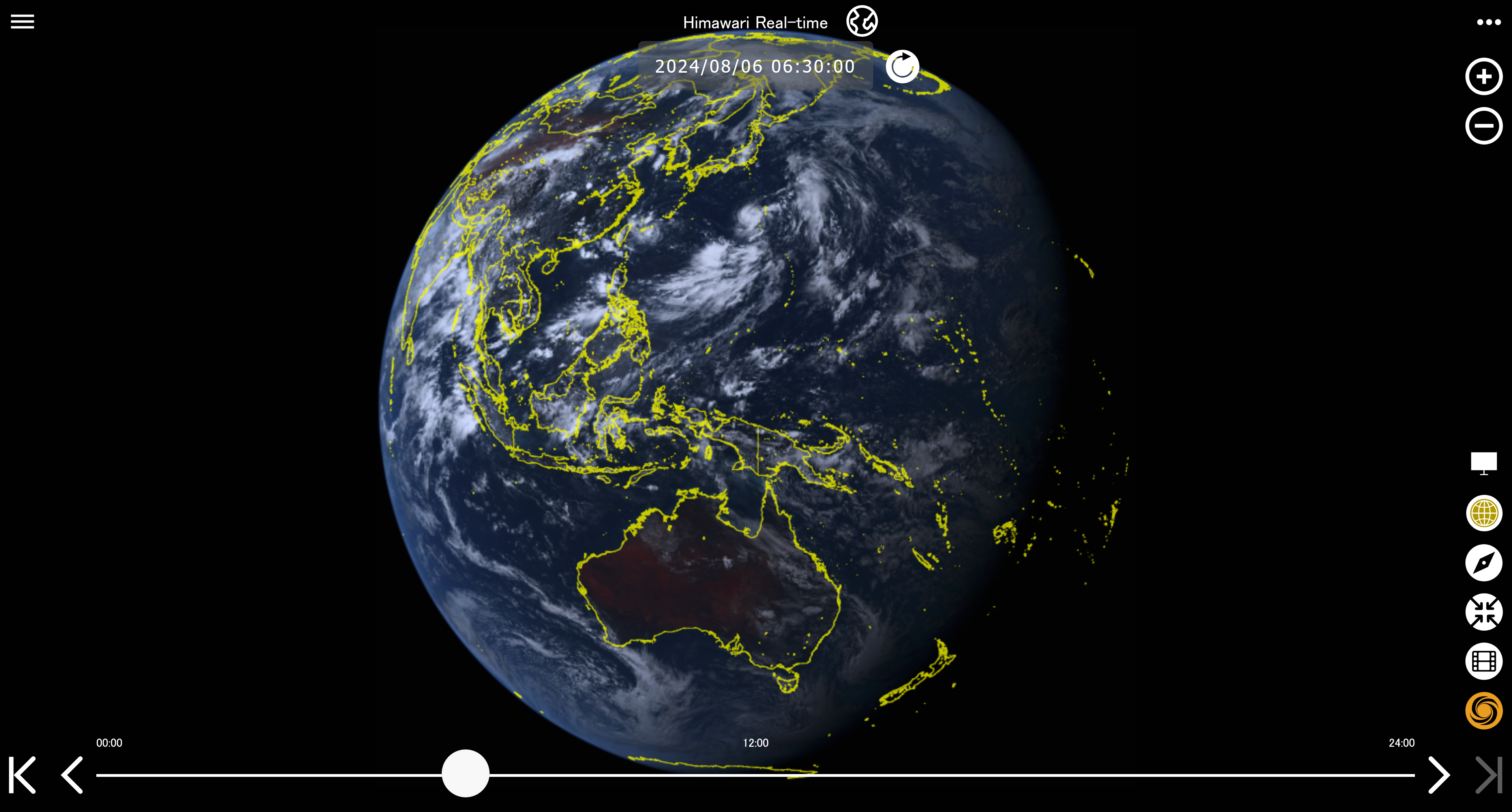
<figure><img src="https://2217084004-files.gitbook.io/~/files/v0/b/gitbook-x-prod.appspot.com/o/spaces%2Fu8dgiMF2h4KnqrWKVkMS%2Fuploads%2F4qTcKey5i9lapIewJYM9%2Fimage.png?alt=media&#x26;token=0f11bf42-3633-4af6-8852-5227354afee5" alt=""><figcaption><p>View from geostationary meteorological Himawari satellite. Credit: NICT, Japan</p></figcaption></figure>

This leads us to **temporal resolution** – the frequency of image update, or revisit time. This frequency depends on orbit geometry, sensor field of view, and local conditions (for example, no optical images in the visible part of spectra are taken during the polar night).

### Optical Remote Sensing and Passive Sensors

Optical sensors are designed to capture radiation in pre-defined spectral intervals, called bands or channels. The image below shows the distribution of spectral bands across optical part of spectra for Sentinel-2, Landsat-7 & 8. You may notice, that spectral bands are designed to insure 1) differentiation between various objects and/or study of their properties and 2) transparency of Earth's atmosphere for outgoing radiation. The human eye sees the interval between 380 and 780 nm (from violet to red). Satellites usually have at least 3 bands in this interval: Blue, Green, and Red - to create a "True-colour" view.

<figure><img src="https://2217084004-files.gitbook.io/~/files/v0/b/gitbook-x-prod.appspot.com/o/spaces%2Fu8dgiMF2h4KnqrWKVkMS%2Fuploads%2Fqm9lL1bxmIHUjRPmECjP%2FSpectral-bands-of-Sentinel-2-and-Landsat-7-8-Spectral-signatures-of-vegetation.jpg?alt=media&#x26;token=38ad5e43-6b2f-4ea8-988e-d30ea5f1deb8" alt=""><figcaption><p>Spectral bands of Sentinel-2 and Landsat 7 &#x26; 8.<br>Spectral signatures of vegetation, soil, and water are depicted in green, red, and blue respectively.<br>Credit: DOI:<a href="http://dx.doi.org/10.13140/RG.2.2.20077.54245">10.13140/RG.2.2.20077.54245</a></p></figcaption></figure>

**Optical sensors features**

| Sensor               | Spectral Bands (Number of bands/ Spectral interval, nm) | Spatial Resolution, m | Revisit time (in December over South Rothera) |
| -------------------- | ------------------------------------------------------- | --------------------- | --------------------------------------------- |
| Sentinel-3 (OLCI)    | 21 / 400-1020                                           | 300                   | 3 times a day                                 |
| MODIS (Terra & Aqua) | 36 / 405 - 965, 3000-15000                              | 250, 500, 1000        | 2 times a day                                 |
| Sentinel-2           | 13 / 443 - 2190                                         | 10, 20, 60            | once in 3 days                                |
| Landsat 8&9          | 11 / 430 -1380, 10600 - 12510                           | 15, 30, 100           | once in 3 days                                |
| Maxar WorldView-3    | 16 / 400 - 1040, 1195 - 2365                            | 0.3, 1.24, 3.70       |                                               |
| Airbus Pleiades      | 6 / 400 - 880                                           | 0.3, 1.2              |                                               |

### Radar Remote sensing and SAR

Another group of imagery we usually work with is SAR (Synthetic Aperture Radar). SAR technology differs greatly in imagery creation methods, wavelengths, and viewing geometry. This makes it more challenging to use, but it has some advantages.

**Active sensors**

While optical sensors measure reflected radiation from the Earth's surface from Sun, radar emits a pulse of microwave energy (wavelengths are cm to tens of cm) and detects its reflection from objects. This means that a) SAR sensors are not light-dependent, as they register their own emitted signal; b) microwave signals can go through clouds, as wavelengths are longer then water particles size.

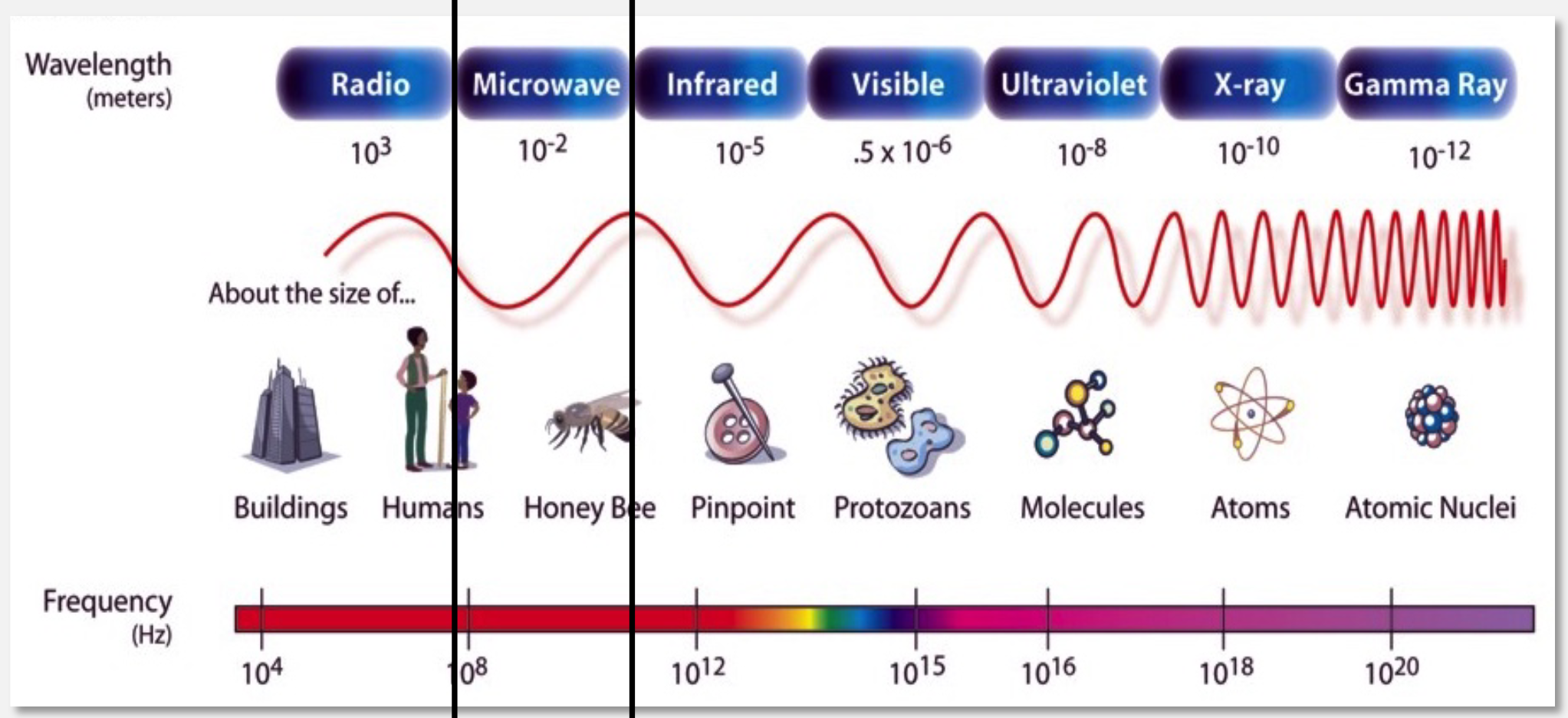
<figure><img src="https://2217084004-files.gitbook.io/~/files/v0/b/gitbook-x-prod.appspot.com/o/spaces%2Fu8dgiMF2h4KnqrWKVkMS%2Fuploads%2F87KG8uIXgLPGUolimwYm%2Fimage.png?alt=media&#x26;token=d8bce937-a077-4bf6-bd62-46e70ecd56fb" alt=""><figcaption><p>Electromagnetic spectrum<br>Credit: NASA ARSET</p></figcaption></figure>

**Wavelengths**

<figure><img src="https://2217084004-files.gitbook.io/~/files/v0/b/gitbook-x-prod.appspot.com/o/spaces%2Fu8dgiMF2h4KnqrWKVkMS%2Fuploads%2FQuFodGEghOoGW1u4lNoj%2Fimage.png?alt=media&#x26;token=6fc559ff-2f47-4fc1-afe7-5975f18740b5" alt=""><figcaption><p>Credit: <a href="https://www.earthdata.nasa.gov/learn/backgrounders/what-is-sar">NASA EarthData</a></p></figcaption></figure>

**Image formation**

Radar registers 3 parameters

* Amplitude - the strength of the reflected echo\
  Amplitude changes due to:
  * Object size and orientation to signal
  * Surface roughness
  * Dielectric properties of the surface
  * Incidence angle
  * Polarization
  * Frequency or Wavelength
* Signal phase
* The time between the pulse generated and the echo received

The latter parameter leads to the necessity of the sensor to look sideways. In another case, two objects at the same distance from the sensor would send the signal back at the same time. This would make it impossible to differentiate them, and therefore, to form an image.

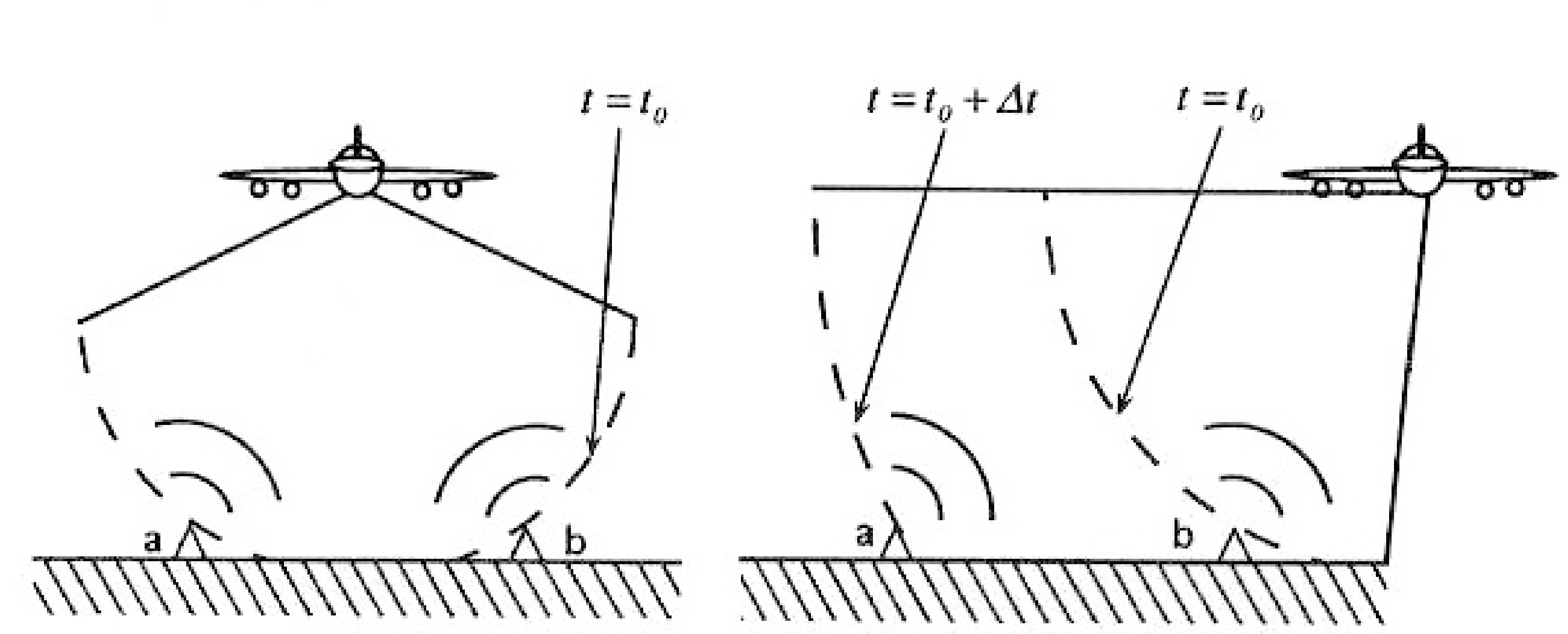
<figure><img src="https://2217084004-files.gitbook.io/~/files/v0/b/gitbook-x-prod.appspot.com/o/spaces%2Fu8dgiMF2h4KnqrWKVkMS%2Fuploads%2FHkYfWgf1PiKmolCCg9x7%2Fimage.png?alt=media&#x26;token=64496a6a-068b-4e8b-bf78-01c171e4a272" alt=""><figcaption><p>Down-Looking vs. Side-Looking Radar<br>Credit: NASA ARSET</p></figcaption></figure>

Sideways-looking geometry plus physical properties of radar wave result in geometrical distortions, known as **Layover** and **Foreshortening**.

Another feature of SAR images is **Speckle** - a specific noise-like pattern, which is a result of interference from the many scattering echoes within a resolution cell.

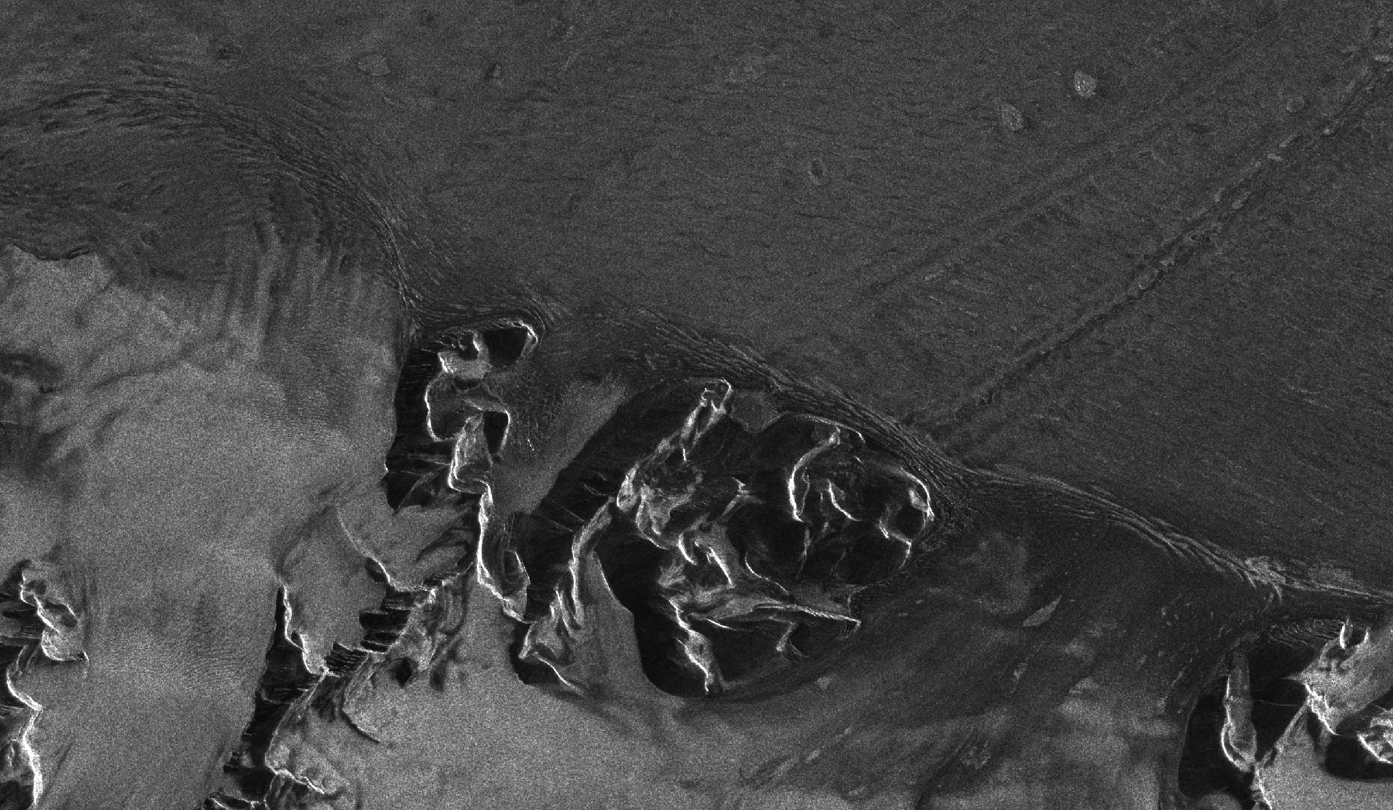
<figure><img src="https://2217084004-files.gitbook.io/~/files/v0/b/gitbook-x-prod.appspot.com/o/spaces%2Fu8dgiMF2h4KnqrWKVkMS%2Fuploads%2FojfOHMfn15d7UtSPb63p%2Fimage.png?alt=media&#x26;token=d8be6da7-8f34-4da3-bdae-7ba0a08b7c68" alt=""><figcaption><p>SAR image, representing Foreshortening, Layover and Shadow effects</p></figcaption></figure>

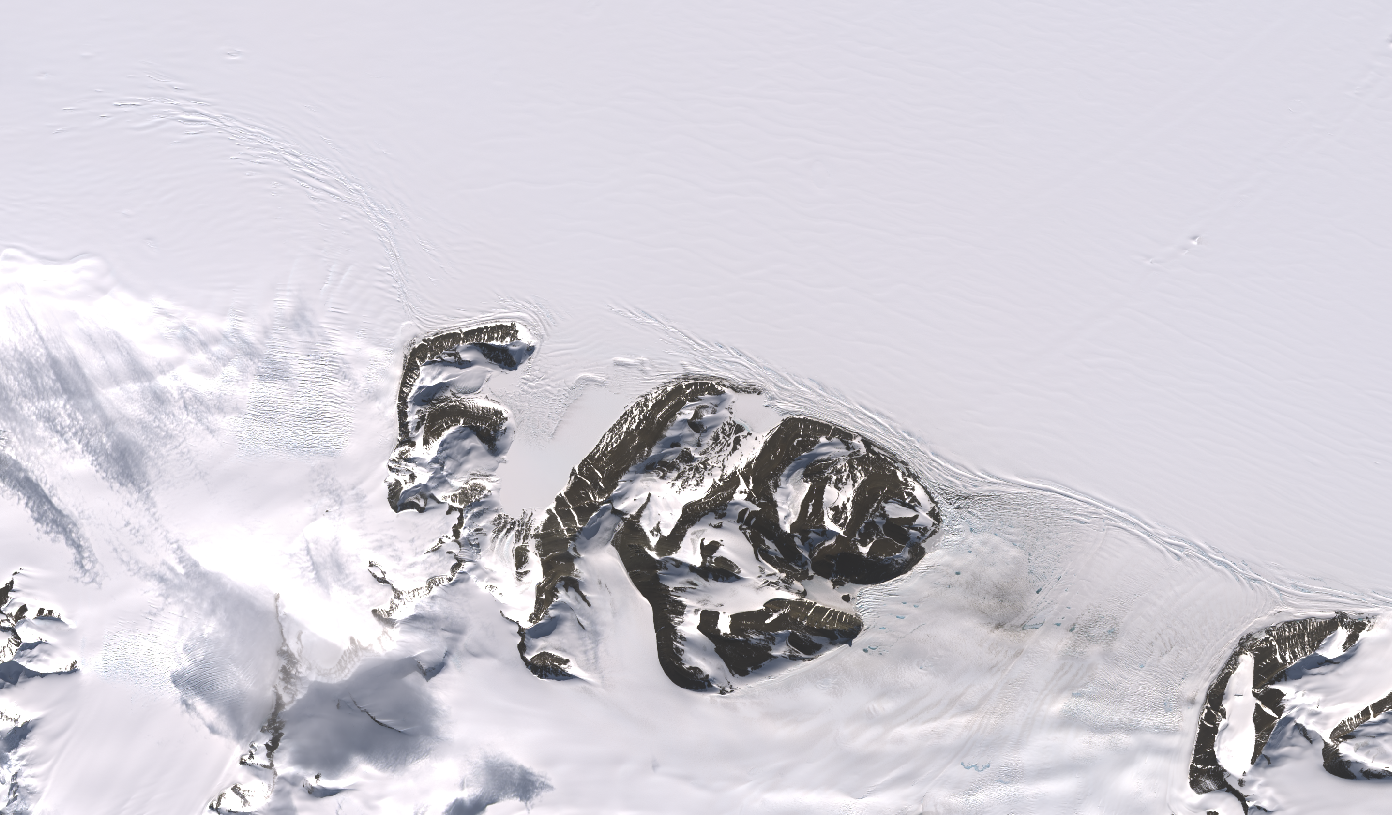
<figure><img src="https://2217084004-files.gitbook.io/~/files/v0/b/gitbook-x-prod.appspot.com/o/spaces%2Fu8dgiMF2h4KnqrWKVkMS%2Fuploads%2Fgq7zTstgYYL07UqtQpB4%2Fimage.png?alt=media&#x26;token=1c753994-9bea-4ccf-8e3d-952a12ba15ee" alt=""><figcaption><p>Optical image</p></figcaption></figure>

### Where do I get a satellite image?

{% hint style="info" %}
Email **<magic@bas.ac.uk>** for any imagery request
{% endhint %}

* **View and download data**
  * Polar View <https://www.polarview.aq/> - latest SAR (Sentinel-1 and RCM) data
  * Copernicus Browser <https://browser.dataspace.copernicus.eu/> - optical and SAR medium-resolution images
  * EO-browser <https://apps.sentinel-hub.com/eo-browser/> - optical and SAR medium-resolution images
  * USGS viewer <https://earthexplorer.usgs.gov/>
* **Any online maps (Google, Bing, ESRI)** - may contain outdated images
* For VHR optical or SAR images **<magic@bas.ac.uk>**

## Image interpretation examples

This page represents some examples of image interpretation

### **Crevassing** <a href="#crevassing" id="crevassing"></a>

* Visible on medium to VHR imagery
* As always with optical: cloud free required
* Low sun angle can be advantageous

<figure><img src="https://guides.geospatial.bas.ac.uk/ops-eo-extention/~gitbook/image?url=https%3A%2F%2F2217084004-files.gitbook.io%2F%7E%2Ffiles%2Fv0%2Fb%2Fgitbook-x-prod.appspot.com%2Fo%2Fspaces%252Fu8dgiMF2h4KnqrWKVkMS%252Fuploads%252FEQjE6smDkfXMzvIyGkXM%252Fcrevassing_Sentinel-2.png%3Falt%3Dmedia%26token%3D890a9cdd-127d-4114-bd22-378dcf77bab5&#x26;width=768&#x26;dpr=4&#x26;quality=100&#x26;sign=cd39a5a8&#x26;sv=2" alt=""><figcaption></figcaption></figure>

Crevassing in McCallum pass, Sentinel-2 Image, Copernicus Sentinel Data 2023, Processed by ESA

<figure><img src="https://guides.geospatial.bas.ac.uk/ops-eo-extention/~gitbook/image?url=https%3A%2F%2F2217084004-files.gitbook.io%2F%7E%2Ffiles%2Fv0%2Fb%2Fgitbook-x-prod.appspot.com%2Fo%2Fspaces%252Fu8dgiMF2h4KnqrWKVkMS%252Fuploads%252FxyinPoODFYNpsVOQ2zYh%252Fcrevassing_Google.png%3Falt%3Dmedia%26token%3De1d5e458-9cc1-42b8-a2ba-2c6562afb68c&#x26;width=768&#x26;dpr=4&#x26;quality=100&#x26;sign=f18e5d2f&#x26;sv=2" alt=""><figcaption></figcaption></figure>

Same area, Google Maps (2024), VHR image.

<figure><img src="https://guides.geospatial.bas.ac.uk/ops-eo-extention/~gitbook/image?url=https%3A%2F%2F2217084004-files.gitbook.io%2F%7E%2Ffiles%2Fv0%2Fb%2Fgitbook-x-prod.appspot.com%2Fo%2Fspaces%252Fu8dgiMF2h4KnqrWKVkMS%252Fuploads%252FwkyZYZFCkJd2TgDATmMh%252Fcrevassing_Umbra.png%3Falt%3Dmedia%26token%3Dfffebe24-5124-4d53-bc65-ff7087ac2dbd&#x26;width=768&#x26;dpr=4&#x26;quality=100&#x26;sign=2ae6ae1&#x26;sv=2" alt=""><figcaption></figcaption></figure>

Same area, Data derived from SAR © \[2024] Umbra Lab, Inc. (originally licensed under CC BY 4.0 )

### **Wildlife** <a href="#wildlife" id="wildlife"></a>

<figure><img src="https://guides.geospatial.bas.ac.uk/ops-eo-extention/~gitbook/image?url=https%3A%2F%2F2217084004-files.gitbook.io%2F%7E%2Ffiles%2Fv0%2Fb%2Fgitbook-x-prod.appspot.com%2Fo%2Fspaces%252Fu8dgiMF2h4KnqrWKVkMS%252Fuploads%252F1TUZlrawiyQE8LyY2Ih3%252FSLH_NEWS16_high_resolution_image_of_emperor_penguin_huddle.jpg%3Falt%3Dmedia%26token%3Dedbfd1e9-97fa-45d3-ae64-1e4f6fdd54bd&#x26;width=768&#x26;dpr=4&#x26;quality=100&#x26;sign=97b2aaa7&#x26;sv=2" alt=""><figcaption></figcaption></figure>

A VHR image of an emperor penguin colony at Halley Bay. An estimated 22,510 penguins were counted at this site. Maxar image, courtesy of the Australian Antarctic Division. [Source](https://www.sciencelearn.org.nz/images/2759-image-of-an-emperor-penguin-colony)

<figure><img src="https://guides.geospatial.bas.ac.uk/ops-eo-extention/~gitbook/image?url=https%3A%2F%2F2217084004-files.gitbook.io%2F%7E%2Ffiles%2Fv0%2Fb%2Fgitbook-x-prod.appspot.com%2Fo%2Fspaces%252Fu8dgiMF2h4KnqrWKVkMS%252Fuploads%252F3rAKCLUqk8X0gAnAfoiw%252Fimage.png%3Falt%3Dmedia%26token%3D8ef013cb-844a-426c-8a41-b97c2893930d&#x26;width=768&#x26;dpr=4&#x26;quality=100&#x26;sign=4e65b14d&#x26;sv=2" alt=""><figcaption></figcaption></figure>

Atka Bay penguin colony on a VHR SAR image. You can see ice on the left and smooth ice, probably covered with fresh snow on the right. White swarms on ice are penguins. Same area, Data derived from SAR © \[2024] Umbra Lab, Inc. (originally licensed under CC BY 4.0 )

### **Sastrugi** <a href="#sastrugi" id="sastrugi"></a>

<figure><img src="https://guides.geospatial.bas.ac.uk/ops-eo-extention/~gitbook/image?url=https%3A%2F%2F2217084004-files.gitbook.io%2F%7E%2Ffiles%2Fv0%2Fb%2Fgitbook-x-prod.appspot.com%2Fo%2Fspaces%252Fu8dgiMF2h4KnqrWKVkMS%252Fuploads%252FP7Tp4Epn9NQjvBYQch9b%252Fimage.png%3Falt%3Dmedia%26token%3D11c70e42-69f1-4cfe-a22d-85de7ca40495&#x26;width=768&#x26;dpr=4&#x26;quality=100&#x26;sign=a39656b4&#x26;sv=2" alt=""><figcaption></figcaption></figure>

Sastrugi on Landsat8 image (15 m)

### **Sea ice** <a href="#sea-ice" id="sea-ice"></a>

#### **Fast ice** <a href="#fast-ice" id="fast-ice"></a>

<figure><img src="https://guides.geospatial.bas.ac.uk/ops-eo-extention/~gitbook/image?url=https%3A%2F%2F2217084004-files.gitbook.io%2F%7E%2Ffiles%2Fv0%2Fb%2Fgitbook-x-prod.appspot.com%2Fo%2Fspaces%252Fu8dgiMF2h4KnqrWKVkMS%252Fuploads%252FWkbk464Tqe2IU7oRQ7LT%252FCase_Corner_2024-03-01_Sentinel-2_L1C_Highlight_Optimized_Natural_Color.jpg%3Falt%3Dmedia%26token%3D530165f7-09ab-46e2-949a-63e201424f68&#x26;width=768&#x26;dpr=4&#x26;quality=100&#x26;sign=c5f3e438&#x26;sv=2" alt=""><figcaption></figcaption></figure>

First-year fast-ice at Case Corner, Modified Copernicus Sentinel data, 2024/Sentinel Hub

<figure><img src="https://guides.geospatial.bas.ac.uk/ops-eo-extention/~gitbook/image?url=https%3A%2F%2F2217084004-files.gitbook.io%2F%7E%2Ffiles%2Fv0%2Fb%2Fgitbook-x-prod.appspot.com%2Fo%2Fspaces%252Fu8dgiMF2h4KnqrWKVkMS%252Fuploads%252F3vloghxHHU8zpiIeAdmC%252F2024-03-11-00_00_2024-03-11-23_59_Sentinel-1_AWS-EW-HH_HH_-_decibel_gamma0.jpg%3Falt%3Dmedia%26token%3Dd64616f4-eef6-4f6f-8ec0-7499218eae5e&#x26;width=768&#x26;dpr=4&#x26;quality=100&#x26;sign=99480fcb&#x26;sv=2" alt=""><figcaption></figcaption></figure>

First-year fast-ice at Case Corner, Modified Copernicus Sentinel data, 2024/Sentinel Hub

#### Pack ice <a href="#pack-ice" id="pack-ice"></a>

<figure><img src="https://guides.geospatial.bas.ac.uk/ops-eo-extention/~gitbook/image?url=https%3A%2F%2F2217084004-files.gitbook.io%2F%7E%2Ffiles%2Fv0%2Fb%2Fgitbook-x-prod.appspot.com%2Fo%2Fspaces%252Fu8dgiMF2h4KnqrWKVkMS%252Fuploads%252FUI3Qmir3BO3qHdtllkQq%252FStangeIceFront_2024-01-07_Sentinel-2_L2A_Highlight_Optimized_Natural_Color.jpg%3Falt%3Dmedia%26token%3D15e00427-a864-40f4-b312-ee09d9f799a1&#x26;width=768&#x26;dpr=4&#x26;quality=100&#x26;sign=12968d29&#x26;sv=2" alt=""><figcaption></figcaption></figure>

Pack Ice and close drift ice at Stange Ice Front, Modified Copernicus Sentinel data, 2024/Sentinel Hub

<figure><img src="https://guides.geospatial.bas.ac.uk/ops-eo-extention/~gitbook/image?url=https%3A%2F%2F2217084004-files.gitbook.io%2F%7E%2Ffiles%2Fv0%2Fb%2Fgitbook-x-prod.appspot.com%2Fo%2Fspaces%252Fu8dgiMF2h4KnqrWKVkMS%252Fuploads%252FHfxzP47yek9EBEfzCnjf%252FStangeIceFront_2024-01-11_Sentinel-1_AWS-EW-HH_HH_-_decibel_gamma0.jpg%3Falt%3Dmedia%26token%3Da16d3326-7fa2-45ae-8d0f-7377823fab0d&#x26;width=768&#x26;dpr=4&#x26;quality=100&#x26;sign=5e306f36&#x26;sv=2" alt=""><figcaption></figcaption></figure>

Pack Ice and close drift ice at Stange Ice Front, Modified Copernicus Sentinel data, 2024/Sentinel Hub

<figure><img src="https://guides.geospatial.bas.ac.uk/ops-eo-extention/~gitbook/image?url=https%3A%2F%2F2217084004-files.gitbook.io%2F%7E%2Ffiles%2Fv0%2Fb%2Fgitbook-x-prod.appspot.com%2Fo%2Fspaces%252Fu8dgiMF2h4KnqrWKVkMS%252Fuploads%252Fc5kONNqM6wJVdwhYuUCi%252Fimage.png%3Falt%3Dmedia%26token%3Dc127183d-bea7-4553-b997-faaf2207aeea&#x26;width=768&#x26;dpr=4&#x26;quality=100&#x26;sign=8cb3bfeb&#x26;sv=2" alt=""><figcaption></figcaption></figure>

Sea ice around Coronation Island, Sentinel-1 SAR (40m, HH polarization) Tabular bergs (bright white) within mobile sea ice. Dense pack ice (up to 100%) with floes bottom-right corner. Open water in the lee of tabular bergs and Coronation Island towards top of image. Open water (dark) left of image. Ice bergs (bright dots) bottom-left of image.


---

# Agent Instructions: Querying This Documentation

If you need additional information that is not directly available in this page, you can query the documentation dynamically by asking a question.

Perform an HTTP GET request on the current page URL with the `ask` query parameter:

```
GET https://guides.geospatial.bas.ac.uk/ops_training/qgis-for-operations/vectors-and-rasters.md?ask=<question>
```

The question should be specific, self-contained, and written in natural language.
The response will contain a direct answer to the question and relevant excerpts and sources from the documentation.

Use this mechanism when the answer is not explicitly present in the current page, you need clarification or additional context, or you want to retrieve related documentation sections.